
We use cookies to ensure our website works properly and to personalise your experience. Cookies policy
Department of Computer Science and Engineering Government Engineering College, Wayanad Kerala, India?
Sickle cell disease (SCD) is a blood disorder characterized by sickle hemoglobin (HbS). Patients suffering from this disease experience acute pain episodes and infections in addition to other chronic conditions like anemia, cardiac, pulmonary, renal and brain complications. The medical field has made great advances in reducing mortality from SCD, but much work remains to be done in improving quality of life for patients. The mechanical properties of individual RBCs in Sickle Cell disease have not been fully assessed, largely due to the limitations of the measurement techniques. Digital Image Processing provides different techniques for the identification of shape and size of cells present in blood. Convolutional Neural Network is one among them. Convolutional Neural Networks (CNNs) are highly effective for image processing due to local receptive fields. CNNs use convolutional layers that apply filters (or kernels) to local regions of the image. This allows the network to detect simple features like edges, textures, or shapes, which can later be combined to recognize more complex patterns. Each filter scans across the image, preserving the spatial relationships between pixels, which is essential for understanding visual data. CNNs learn hierarchical patterns, from low-level features (like edges) in the first layers to more abstract and complex features (like faces or objects) in the deeper layers. This makes them very powerful for tasks like object recognition, classification, and detection. This project deals with designing a system for detecting the shape of deformed cells within seconds with higher accuracy.
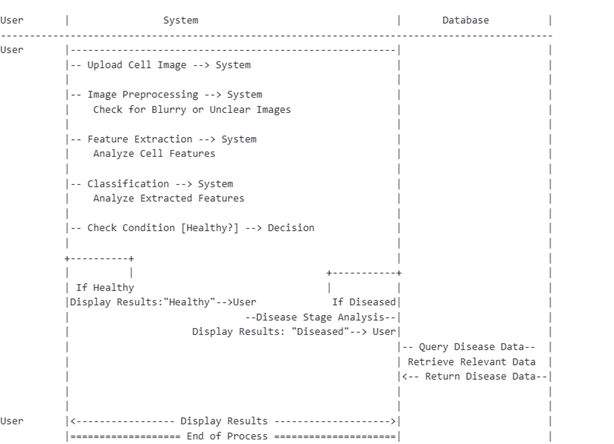
Sickle cell anemia is a genetic blood disorder that affects the shape and function of red blood cells. In a healthy person, red blood cells are round and flexible, allowing them to flow smoothly through blood vessels. However, in people with sickle cell anemia, these cells are shaped like a crescent or sickle. Image processing techniques can be used to differentiate between sickle cells and normal red blood cells by analyzing various visual features such as shape, size, and color. These methods can significantly aid in improving diagnostic accuracy and streamlining medical workflows. Employing advanced algorithms can help identify abnormalities with greater speed and precision. Furthermore, such tools can assist researchers in studying the disease?s progression and evaluating the effectiveness of treatments. This flowchart describes an image processing pipeline for sickle cell anemia detection and classification in medical diagnosis scenario.
?? ? ? ?
? ? ? ? ? ? 
? ? ? ?
Fig. 1. Flow chart
Start: The process begins.
Upload image: The system first requires an RBC image to be uploaded.
Image pre-processing: The uploaded image undergoes pre- processing, which may involve operations like noise reduction, resizing, contrast adjustment, or other enhancements to improve the quality of the image for further analysis.
Feature extraction: Important features are extracted from the pre-processed image. Features could include texture, color, shapes, or any other distinctive attributes that help identify whether the image represents a defect or disease.
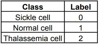
Classification: Based on the extracted features, the image is classified using CNN algorithm. RBCs can be classified into normal cell, sickle cell and thalassemia cell. The classification determines whether the RBC in the image has a ?defect? (sickle cell anemia/ thalassemia) or not. High-resolution images of the red blood cells are collected from SCDIR (Sickle Cell Disease Image Repository). This is a specialized repository for sickle cell-related data. It includes images of blood smears showing both sickle-shaped and normal red blood cells. The data set includes 3 classes; Normal cell, Sickle cell and Thalassemia cell. Both sickle cell anemia and thalassemia are inherited blood disorders that affect hemoglobin production and lead to anemia, but they are caused by different genetic mutations. Image pre-processing is done in order to enhance the quality of the image and makes it ready for analysis. Deep learning technique called CNN (Convolutional Neural Network) is used to classify the images. CNNs can automatically learn features from the images without manual feature extraction [1]. After training on labeled data (sickle vs. normal cells vs. thalassemia), CNNs can classify cells with high accuracy. The goal is to develop a system that can distinguish the characteristic crescent or sickle shape of red blood cells seen in sickle cell anemia from the normal disc-shaped cells.
? ? ? ?
? ? ? ? ? ? 
? ? ? ?
Fig. 2. System architecture
A popular Convolutional Neural Network (CNN) architecture VGG16 is designed to handle high-resolution images. The small 3x3 convolutional filters used by VGG16 capture fine details and patterns, making it effective at detecting slight deformations in red blood cells. To manage and process the large-scale dataset of the RBCs, Google Colab is used. Google Colab can provide robust computational resources through its provision of free access to GPUs and TPUs. This access is crucial for performing the computationally intensive tasks associated with training and evaluating deep learning models.
? ? ? ?
? ? ? ? ? ? 
? ? ? ?
Fig. 3. Sequence diagram
II.??????? METHODOLOGY
A.??????? Convolutional Neural Network
Convolutional Neural Networks (CNNs) are a type of deep learning technology. They are a specialized kind of neural network designed to process and analyze data with grid-like topology, particularly for image processing tasks. CNN consists of several layers, including convolutional layers, pooling layers, fully connected layers, and activation layers. CNN eliminates the need for manual feature extraction, which is crucial for detecting subtle shape changes in sickle cells. As the network deepens, it starts learning more complex patterns, such as cell contours and inner texture variations, which are useful in identifying abnormal cells. Sickle cells can appear in different orientations (rotated, flipped) in blood smear images. CNN can handle this variability due to the properties of convolutional layers, which detect features regardless of their position or orientation in the image. CNN uses back-propagation to adjust the weights by calculating the error gradient. Pooling layers reduce the spatial dimensions of feature maps while retaining the most important information. This ensures that the model focuses on critical features such as the irregular shape or pointed ends of sickle cells, while discarding irrelevant background information.
1)???????? Model Description: Pre-trained models like ResNet or VGG16 can be fine-tuned on the sickle cell dataset to enhance performance with smaller datasets. VGG16 is designed to handle high-resolution images which helps in identifying small and subtle features. It consists a small 3x3 convolutional filter that detect slight deformations in red blood cells. VGG16 works well with various image processing techniques such as image augmentation (rotation, zoom, shift, flip, translation, scale, shear, crop, color jittering) and normalization. With proper tuning and dataset-specific training, VGG16 can achieve high accuracy in distinguishing normal RBCs from sickle cells. There are three classes in this experiment and requires a Multi-Class Classification.
? ? ? ?
? ? ? ? ? ? 
? ? ? ?
A label is the actual value or category that the model is supposed to predict for each input example. Labels can be binary, multi-class, or continuous depending on the type of problem. The process involves dataset preparation, training, testing and evaluation of the model. Implementation was done in Google Colab to speed up training and inference processes significantly.
2)???????? Data pre-processing: Data preprocessing is done to prepare raw data for analysis or model training. Preprocessing ensures that the data is in a suitable format for the model and significantly improve model accuracy and performance. For classifying RBCs using VGG16, preprocessing ensures that the images are standardized, noise is reduced, and important features (such as the shape of cells) are retained. VGG16 requires a fixed input size for images. Image resizing libraries (e.g., OpenCV, PIL) are used to ensure that all RBC images match the input size required by VGG16. The input to VGG16 is an image of size 224x224 pixels with three color channels (RGB). All images in the dataset need to be resized to this fixed size [1]. Pixel values in images typically range from 0 to 255. Normalizing these values to a range between 0 and 1 can help improve the training process and prevent numerical instability in deep learning models. Divide the pixel values by 255 to scale them into the range of [0,1]. Since medical datasets like RBC images are often small, data augmentation techniques are used to artificially increase the size of the dataset and improve model generalization. This can help VGG16 recognize RBCs in different orientations or under varied conditions. Transformations such as rotation, flip- ping, shifting, zooming, or brightness adjustment are applied.
Blood smear images may contain noise such as background artifacts or image distortions. Reducing noise can improve the quality of input images, making it easier for VGG16 to learn distinguishing features between normal, sickle cells and thalassemia cells. Filters such as Gaussian blur or median filters can be used to smooth out the noise. If the dataset is imbalanced, techniques like oversampling or under-sampling can be used to balance the classes. Over-sampling can generate synthetic minority class samples, while under-sampling can reduce the majority class to improve balance. By balancing the dataset, these techniques prevent the model from being biased toward the majority class, ensuring that it can learn to recognize both normal cells and defective cells effectively.
B.???????? Experimental setup
The proposed model for detecting sickle cell anemia was developed and trained using the Google Colab platform. Google Colab can provide numerous advantages, especially in handling deep learning models, large datasets, and resource- intensive computations. Google Colab provides free access to powerful hardware such as GPUs (Graphics Processing Units) and TPUs (Tensor Processing Units). VGG16 requires significant computational power and utilizing Colab?s GPU/TPU can drastically speed up model training and testing, for image processing tasks. Google Colab supports easy integration with Google Drive, allowing seamless access to large datasets. This is particularly useful if the local system cannot handle large volumes of data or storage is limited. Google Colab makes it easy to import popular libraries like TensorFlow and Keras, which come with access to pre-trained models such as VGG16. Using Colab allows to leverage these models for transfer learning, significantly reducing the time and resources needed to train from scratch.
Colab allows to share notebook with collaborators easily. All experiments, code, and results are saved in a single notebook, ensuring that the entire experimental setup is re- producible. Colab can handle multiple training runs and hyper-parameter tuning without the need for local computational resources. This allows to perform extensive experiments on deep learning models, adjusting architectures, learning rates, optimizers, and data augmentation techniques without performance bottlenecks. It also supports libraries like OpenCV, PIL, and TensorFlow, which are crucial for preprocessing images in sickle cell detection. It is possible to perform data augmentation, resizing, normalization, and other transformations needed to enhance the quality of the dataset and improve model performance. Google Colab supports visualization libraries such as Matplotlib, Seaborn, and TensorBoard to help visualize training progress, accuracy, loss, and other key metrics. Data visualization tools help in understanding model performance and predictions.
C.???????? Training
SCDIR (Sickle Cell Disease Image Repository) is used for collecting required dataset. The dataset is then split into training, validation, and test sets to ensure that the model generalizes well on unseen data. Dataset was divided as 80 percent for training, 10 percent for validation, and 10 percent for testing. If the dataset is large and cannot fit into memory, batch processing can be used to load a subset of images into memory during training. Ensure that the dataset is properly labeled. Fine-grained labels are used to distinguish between sickle cells and thalassemia cells. Use a pre-trained CNN like VGG16 to take advantage of transfer learning. The model is trained on large datasets like ImageNet and can be easily fine- tuned for sickle cell classification. For fine-tuning, remove or modify the final fully connected layers of the pre-trained model to adapt it to the number of classes. An appropriate loss function should be chose based on the task. For multi-class classification, categorical cross-entropy is used. Optimizer like Adam adjusts learning rates dynamically during training, leading to faster convergence. Define the batch size (e.g., 32 or 64), depending on the available computational resources and set the number of epochs (iterations over the entire dataset) for training. Applying dropout layers in the model can prevent overfitting. Stop training once the validation loss stops improving.
D.??????? Model evaluation
Model evaluation is the process of assessing how well a trained model performs on unseen data. The purpose is to measure the model?s generalization ability and to ensure that it meets the performance requirements of the task. It involves using various performance metrics and methods to understand how accurately and effectively the model can make predictions based on cell images. Model evaluation allows to detect potential issues like overfitting, underfitting, or biases in the model. It also helps in comparing different models or model configurations to select the best one.
1)???????? Performance metrics: In deep learning tasks like image classification, it?s important to have quantifiable metrics to measure success. Model evaluation allows to compute these metrics, such as accuracy, precision, recall, F1-score, AUC- ROC for classification tasks. The model does not typically update its weights after seeing each individual sample. Instead, the dataset is divided into smaller groups called batches. The batch size determines how many samples the model processes before updating its weights.
? ? ? ?
? ? ? ? ? ? 
? ? ? ?
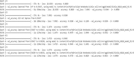
Once all batches in the dataset have been processed, one epoch is completed. An epoch refers to one complete pass of the entire training dataset through the model. The model is trained for several epochs to adjust its parameters. Initially, in Epoch 1, the training accuracy was 0.8029, and the validation accuracy achieved a promising 0.93437, reflecting good generalization early on. In Epoch 2, despite a jump in training accuracy to 0.9260, the validation accuracy did not improve, suggesting the potential onset of slight overfitting. Finally, in Epoch 5, the model achieved its best performance, with training accuracy at 0.9739 and validation accuracy at 0.98333, highlighting excellent generalization capabilities.
? ? ? ?
? ? ? ? ? ? 
? ? ? ?
Fig. 4. Training and validation loss
A graph is generated representing the training loss and validation loss. Both training and validation loss should decrease and ideally converge.
? ? ? ?
? ? ? ? ? ? 
? ? ? ?
Fig. 5. Training and validation accuracy
Training accuracy and validation accuracy are also plotted. During each epoch the Training and validation accuracy im- proves and attained an optimal value at the fifth epoch.
? ? ? ?
? ? ? ? ? ? 
? ? ? ?
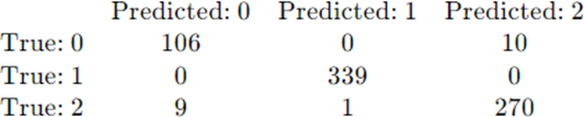
Fig. 6. Confusion matrix
A confusion matrix is generated to evaluate the performance of the classification model. It allows to visualize how well a model classifies different classes by displaying the number of correct and incorrect predictions made by the model. Each row in the matrix represents the actual class, and each column represents the predicted class. The diagonal values represent the number of correctly predicted instances for each class, while the off-diagonal values represent the misclassifications.
? ? ? ?
? ? ? ? ? ? 
? ? ? ?
Fig. 7. Multi-class confusion matrix structure
??????????? True positives (TP)
TP0: Correct predictions for class 0 TP1: Correct predictions for class 1 TP2: Correct predictions for class2
??????????? False positives (FP)
FP0: Instance from class 1 incorrectly classified as 0 FP1: Instance from class 2 incorrectly classified as 0 FP2: Instance from class 2 incorrectly classified as 1
??????????? False negatives (FN)
FN0: Instance from class 0 incorrectly classified as 1 FN1: Instance from class 0 incorrectly classified as 2 FN2: Instance from class 1 incorrectly classified as 2
In Fig.6, 106 instances were correctly classified as sickle cell, 0 were predicted as class 1, and 10 were misclassified as class
2. 339 instances were correctly classified as normal cell, and no misclassifications occurred. 270 instances were correctly classified as Thalassemia cell, but 9 were incorrectly classified as class 0, and 1 as class 1. This matrix helps to find out the performance parameters like accuracy, precision, recall, F1- score etc.
E.???????? Results
For multi-class classification, performance parameters can be computed for each class or averaged across all classes. True Positives (TP), False Positives (FP), False Negatives (FN), and True Negatives (TN) are key values that are used to attain final results. These values identify errors in the model and help understand its performance in each class. Analyzing these metrics helps pinpoint specific areas where the model is underperforming, such as misclassifying certain classes. Additionally, these metrics provide insight for more detailed optimization of the model, enabling adjustments to thresholds.
Accuracy is the ratio of correctly predicted instances (both positive and negative) to the total number of predictions.
?
?
Precision is the ratio of correctly predicted positive instances (true positives) to the total predicted positives.
?
?
Recall is the ratio of correctly predicted positive instances (true positives) to the total actual positives (true positives and false negatives)
?
?
The F1-score is the harmonic mean of precision and recall, providing a balanced measure to account for both false positives and false negatives.
?
? ? ? ?
? ? ? ? ? ? 
? ? ? ?
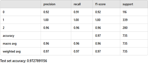
Fig. 8. Performance parameters
In Fig.8 , macro average refers to the unweighted average of a performance metric (such as precision, recall, or F1-score) across all classes in a multi-class classification problem. Each class contributes equally, regardless of the number of samples (support) in that class. Weighted average is the average of a performance metric (such as precision, recall, or F1-score) across all classes, where the contribution of each class is weighted by the number of instances (support) in that class. Classes with more data points have a greater influence on the final metric value. Support refers to the number of actual instances of each class in the dataset. The calculated accuracy of the model VGG16 was 97.2 percentage.
? ? ? ?
? ? ? ? ? ? 
? ? ? ?
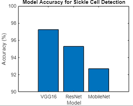
Fig. 9. Comparison of CNN models
The bar chart illustrates the comparative performance of three deep learning models VGG16, ResNet, and MobileNet in detecting sickle cell disease, with their accuracy percentages represented on the vertical axis. The accuracy values range between 90 percent and 100 percent, and the chart highlights the varying performances of the models. Among the three models, VGG16 demonstrates the highest accuracy, achieving close to 97 percent. This indicates its superior ability to identify sickle cell disease with a minimal error rate, making it the most effective model in this study. The high accuracy of VGG16 can be attributed to its robust architecture and extensive feature extraction capabilities, which allow it to accurately capture the complex patterns associated with sickle cell abnormalities. Following VGG16, the ResNet model achieves an accuracy of approximately 95 percent, showcasing competitive performance. ResNet?s relatively high accuracy can be attributed to its deep residual network architecture, which mitigates issues such as vanishing gradients, enabling efficient training of deeper networks. However, its performance still falls slightly short of VGG16, indicating room for further optimization or fine-tuning. In contrast, MobileNet achieves the lowest accuracy among the three models, at approximately 92 percent. While MobileNet?s lightweight architecture makes it well-suited for deployment on mobile and edge devices, its relatively lower accuracy suggests that it may struggle to capture the intricate features needed for precise sickle cell detection. This trade-off between computational efficiency and accuracy highlights the model?s limitations for tasks requiring high precision.
The results indicate that while all three models perform well, VGG16 emerges as the most accurate and reliable model for detecting sickle cell disease. ResNet follows closely behind, and MobileNet, though efficient, lags in accuracy. These findings suggest that for critical applications like sickle cell detection, model accuracy should be prioritized over computational efficiency to ensure reliable results.
REFERENCE


Subhaga K*, Adarsh Dilip Kumar T P, Sickle Cell Anemia Detection Using Deep Learning, Int. J. Sci. R. Tech., 2025, 2 (1), 10-17. https://doi.org/10.5281/zenodo.14591579
 10.5281/zenodo.14591579